How to Use Vlookup Function in Excel 2010 With Example

VLOOKUP for Dummies (or newbies)

VLOOKUP is a powerful and handy excel function. At the same time, it is one of the least understood functions and can often break. Today we'll try to explain VLOOKUP for newbies in the simplest possible way. We'll also provide formula examples of the function's most typical usage.

If you want to skip the text and head straight for a video tutorial, take a look at this Top Ten Formulas and Functions in Excel tutorial that we held.

Excel VLOOKUP Function – Syntax and Primary uses
- What is VLOOKUP?
- VLOOKUP Syntax
VLOOKUP for Dummies – Video Tutorial
How to Use VLOOKUP in Excel?
- Step 1: Organize your data for VLOOKUP
- Step 2: Set the Lookup Value
- Step 3: Specify where to search
- Step 4: Specify which information you need
- Step 5: Choose between Exact or approximate match
VLOOKUP Examples
- VLOOKUP Example 1
- VLOOKUP Example 2
- VLOOKUP Example 3
Excel Tips on the VLOOKUP Function
Using Wildcards (?,*) in VLOOKUP Formula
- VLOOKUP Wildcard Example 1
FAQs

Related:

SUMIF With Multiple Columns – The SUMIFS Function In Excel

How to Use Goal Seek in Excel? (3 Simple Examples)

How to Use Excel COUNTIFS: The Best Guide

XLOOKUP Google Sheets – 4 Best Alternatives!

Excel VLOOKUP Function – Syntax and Primary uses

What is VLOOKUP?

VLOOKUP is a function that searches for the value you specify. The result returns a matching value from another column. To be more technical, you choose a range, and VLOOKUP looks up the value in the first column. The result it returns is a value from the same row of another column.

The letter "V" in VLOOKUP stands for "vertical." It is there to differentiate from the function HLOOKUP, where the "H" stands for horizontal. HLOOKUP is different that VLOOKUP only in the way that it looks up a value in a row rather than a column.

All versions of Microsoft Excel have the VLOOKUP function available.

VLOOKUP Syntax

The VLOOKUP syntax looks like this:

VLOOKUP(lookup_value, table_array, col_index_num, [range_lookup])

The VLOOKUP function has four arguments. The first three are required, and the last one is optional.

The easiest way to describe it is this:

Lookup_value – what you want to lookup
Table_array – where you want to look for it
Col_index_num- the range containing the value to return
[range_lookup]- returns an approximate or exact match

VLOOKUP for Dummies – Video Tutorial

To see VLOOKUP in action, take a look at the following video:

VLOOKUP for Dummies

How to Use VLOOKUP in Excel?

Using VLOOKUP is very simple. You just need to enter the appropriate values for the four arguments.

To easily use VLOOKUP in Excel follow these simple steps:

Step 1: Organize your data for VLOOKUP

Organize your data properly in the correct order, before using the VLOOKUP formula. Keep in mind that VLOOKUP searches for the data in the right-hand side direction of the lookup value. Hence, make sure that the column that contains the value you need to extract appears after the lookup column.

Step 2: Set the Lookup Value

Now, you need to tell the VLOOKUP formula, what are you looking for. This is the very first argument of the VLOOKUP formula, VLOOKUP(lookup_value, table_array, col_index_num, [range_lookup]). Note that, the lookup value can be directly entered inside the formula, or be referenced as a cell reference.

Step 3: Specify where to search

Next, tell VLOOKUP where to look for the information, i.e. the table array. Do this by highlighting the table which contains the information. You can also manually enter the range of the table array inside the formula.

Step 4: Specify which information you need

Now, you need to specify the column which contains the information you need VLOOKUP to return. Do this, by entering the index number of the column, in the VLOOKUP formula. In simple words, enter the position of the column in the table range. For example, if your desired data is present in the 4th column, then enter Col_index_num as 4.

Step 5: Choose between Exact or approximate match

Finally, you need to tell VLOOKUP if you want an exact match or approximate match for the lookup value. Enter TRUE for approximate match and FALSE for an exact match. By default, it will be set to TRUE if you don't specify anything.

Also Read:

5 Steps To Easily Use Excel 3D Maps (Bonus Video Included)

Create An Excel Dashboard In 5 Minutes – The Best Guide

Excel Dynamic Array: 8 Must-Know Formulas

VLOOKUP Examples

Now, let's see how to implement all these steps with the help of these three examples.

VLOOKUP Example 1

In this example, we have a list of fruit in column A, and the amounts of them in column B. Now imagine having hundreds of items in A and B, and you need to find a specific one.

You do that with VLOOKUP. Let's find the amount of Apples on this list.

What can we see from the formula used?

=VLOOKUP(A8;A2:B5;2;FALSE)

The Syntax is,

VLOOKUP(lookup_value, table_array, col_index_num,[range_lookup])

The first argument is lookup_value, and it's Apples in cell A8.

The second argument is the table_array, and we chose everything from A2 to B5.

The third argument is col_index_num, and we entered "w" because that is the second column in the array.

The fourth argument is [range_lookup], and we entered FALSE, which returns an exact match. Because this argument is optional, if you leave it empty, the default value will be TRUE, and that is the approximate value.

The result ended up being 50, which we can see, is correct.

VLOOKUP Example 2

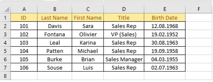
In example 2, we'll try to find the first name of an employee. We know his last name but not his first. In a company with hundreds and thousands of employees, VLOOKUP can be quite useful in finding specific information in this scenario.

Just by looking, we know that we used the VLOOKUP correctly and returned the first name as Olivier.

=VLOOKUP(B3;B2:E7;2;FALSE)

looking at what we did in this formula.

The first argument, lookup_value is B3, we could have manually entered "Fontana" because that was the information we know, but simply clicking on B3 was faster.

The second argument, the table_array, is everything from B2 TO E7.

The third argument, col_index_num, is the number of the column we want to search for. Because we need the first name, we'll enter number 2. If we wanted to find out the title of the employee, we'd type in number 3 because that is the third column in the table_array.

The fourth argument is [range_lookup], and we entered FALSE, which returns an exact match.

VLOOKUP Example 3

For the third example on how to use VLOOKUP, we want to find out what the last name is of the person with ID number 106 is.

=VLOOKUP(A7;A2:E7;2;FALSE)

So what did we do in this VLOOKUP formula?

The first argument is A7 since we are looking for the ID 106.

The second argument, the table_array, is everything from A2 TO E7.

The third argument is the number of the column. The last name is in the second column, so we entered number 2.

And the fourth argument we put FALSE to get an exact match.

We can see that we correctly used the VLOOKUP function and got the correct last name, which is Souse.

Excel Tips on the VLOOKUP Function

The VLOOKUP function cannot look to its left. It always searches the leftmost column of the table_array and returns a value from the column from the right.

2. Keep in mind that the VLOOKUP function is not case-insensitive. That means lowercase and uppercase letters are treated as the same.

3. Don't forget the fourth argument, which is TRUE for an approximate match and FALSE for an exact match. If you don't enter anything, the default value is TRUE.

4. The TRUE value will first look for an exact match, and if it can't find it, it will then look for the next largest value that is less than the lookup value.

5. Data in a column needs to be sorted in ascending order when searching for TRUE (approximate match)
You will get the result #N/A error if the lookup value is not found.

Using Wildcards (?,*) in VLOOKUP Formula

Like in most excel functions, wildcards are available for VLOOKUP as well.

To match any single character, the question mark "?" is used .
The asterisk "*" is used to match any sequence of characters.

Imagine you can't remember the exact text you are looking for, or maybe you are looking for a text string that is part of the cell contents. That's when you use wildcards.

VLOOKUP Wildcard Example 1

In a case where you have a list of hundreds of employees, and you want to find out the particular salary of someone who you can't remember exactly. You know his name begins with an "ack."

Let's search in the database.

=VLOOKUP(I2&"*";A2:B10;1;FALSE)

What did we do in this VLOOKUP formula?

The first argument we clicked on I2, which is "ack" because we know the last name starts with those three letters. And then we added &"*".

& – stands for, and the asterisk searches for everything after the ack.

The second argument is the table array, where we entered everything from A2 to B10.

The third argument is the column we want to return. Since we want to return the last name, that is column 1, and we entered 1.

Just like always, we want the exact match, so we entered FALSE as the fourth argument.

Just by looking, we can see that we used the VLOOKUP function correctly and got the correct result.

To return the salary, we can use the same formula and only change the third argument. That is what column to return. Since the salary is in the second column, we enter 2 as the third argument.

=VLOOKUP(I3&"*";A3:B11;2;FALSE).

If you are looking up data horizontally, instead of vertically, then you need to perform exactly the same as the above, but use HLOOKUP instead of VLOOKUP.

Both VLOOKUP and HLOOKUP work in the same way!

Suggested Reads:

How to Delete a Pivot Table in Excel? 4 Best Methods

How to Enable Excel Dark Mode? 3 Simple Steps

How to Extract an Excel Substring? – 6 Best Methods

FAQs

How to use VLOOKUP in Excel?

Use VLOOKUP in Excel to search for a specified value in a range and return a corresponding value from the range. The VLOOKUP function syntax is VLOOKUP (value, table, col_index, [range_lookup]) where "value" is the value we are searching for. "table" is the data range where we have to search. "col_index" is the index of the column that contains the value which needs to be returned. [range_lookup] specifies if need an exact match or approx. match

What is VLOOKUP used for?

Use VLOOKUP when you need to find a particular kind of information corresponding to a variable from a large sheet. For example, use it when you need to find the phone number of customers when you search for their names, from a sheet that contains all this data in a table.

Take a look at the VLOOKUP killer released by Microsoft – XLOOKUP.

There are so many great resources written on VLOOKUP. One of our favorites is this list of 23 things you should know about VLOOKUP.

To check out the range of Excel courses on Simon Sez IT, go here.

Other Excel classes you might like:

Introduction to Power Pivot & Power Query in Excel
What-If Analysis in Excel
Designing Better Spreadsheets in Excel
Logical Functions in Excel

Deborah Ashby

Deborah Ashby is a TAP Accredited IT Trainer, specializing in the design, delivery, and facilitation of Microsoft courses both online and in the classroom. She has over 11 years of IT Training Experience and 24 years in the IT Industry. To date, she's trained over 10,000 people in the UK and overseas at companies such as HMRC, the Metropolitan Police, Parliament, SKY, Microsoft, Kew Gardens, Norton Rose Fulbright LLP. She's a qualified MOS Master for 2010, 2013, and 2016 editions of Microsoft Office and is COLF and TAP Accredited and a member of The British Learning Institute.

Source: https://www.simonsezit.com/article/vlookup-for-dummies-or-newbies/

Posted by: mcvicarsolike1953.blogspot.com

How to Use Vlookup Function in Excel 2010 With Example